Update: AirGradient and the PM_2.5 correction algorithm from the EPA

Introduction

In September 2024, we published an article about PM_2.5 and how the EPA correction algorithm improves the accuracy of AirGradient’s monitors. We observed that our sensors, the PMS5003 from Plantower, systematically overestimate PM_2.5 when concentrations are above 10 to 20 µg/m³. The algorithm from the EPA ( equation 4) does a great job of bringing down the high readings. Meanwhile, we have implemented the algorithm for our outdoor and indoor monitors, as explained here. Today’s article looks again into the algorithm’s performance based on additional data from our global colocation project.

Overview

We started testing our outdoor OpenAir monitors in 2023 with various reference instruments in various locations around the globe. This effort is only possible thanks to the generous support of numerous local research partners. We are extremely grateful for these ongoing collaborations!

The last blog article (September 2024) covered nine outdoor locations in 6 countries with a total of 19 years of AirGradient PM_2.5 data. Since then, our colocation data has doubled: today’s article covers 17 outdoor locations in 11 countries with 37 years of PM_2.5 colocation data.

The table below provides information about the individual locations and reference instruments. The new locations are highlighted in blue.

* Collocation in Manchester UK took place indoors with six ‘One’ monitors from AirGradient and one ‘Modulair’ from QuantAQ as a reference.

The appendix of this article shows individual scatter plots for every location. It further includes R², intercept, slope, MAE, RMSE, nRMSE, and mean for every single sensor. The raw reference and AirGradient data for all locations will also be available soon in three versions: hourly and daily averages and higher time-resolution where available.

Results

Below are all 12513 daily PM_2.5 data points visualized in a scatter plot. Raw data is shown on the left, and the EPA-corrected data is on the right. This data excludes the Manchester data due to the lack of a FEM reference.

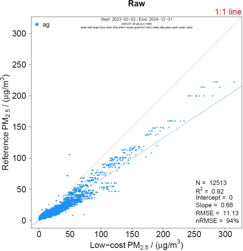
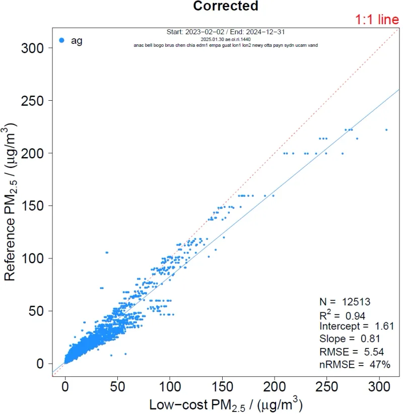
Note that the correlation results shown in the two scatter plots above consider every single data point equally, meaning that locations with more data have more weight on these numbers.

The table below describes the accuracy of our outdoor OpenAir monitors before (‘raw’) and after (‘corrected’) applying the EPA correction algorithm for PM_2.5. It is based on daily averages. The R² value describes how well the AirGradient monitors correlate with the collocated reference instrument – the closer R² is to 1, the stronger the correlation. nRMSE indicates the relative error of the AirGradient monitors, assuming the reference instruments are 100% correct – the lower the nRMSE, the better the agreement. The last column shows whether and by how much the EPA correction algorithm has improved the accuracy of our monitors.

Improvement factor = nRMSE (raw) / nRMSE (corrected)

If the factor is greater than 1, the error of the EPA-corrected measurements is lower than the error of the raw data, i.e. the accuracy has improved, and the larger the improvement factor, the better the improvement. If the factor is below 1 the EPA formula introduces a larger error, i.e. a reduced accuracy.

The mean absolute error (MAE, shown in the appendix) improved from 7 to 3 µg/m³ as a result of the algorithm (average across all sensors). In other words, the differences between the reference and AirGradient readings were, on average 3 µg/m³ (after correction). Note that this metric is greatly influenced by episodes with high PM_2.5 concentrations, so it is not necessarily accurate for low PM_2.5 readings.

In the table above, we find that the average nRMSE improved from 79 % to 38 % upon correction with the EPA algorithm. This is similar to last year’s results (86 % to 34 %). Again, an average improvement factor of 2.5 was found.

While we observed an improved nRMSE in 9 of 9 locations last year, we have found improved factors in only 14 of 17 locations this time. In three locations (Sydney, Guatemala City, and Bogota), we have observed a worsening of the monitor’s accuracy when applying the EPA algorithm and using nRMSE as a metric (daily averages). This prompted us to investigate these locations in more detail.

Sydney (Australia)

We have 122 days of data where an AirGradient OpenAir monitor is collocated in Sydney (Australia) with a Thermo 5014i reference instrument. The scatter plot below shows the 122 days of data (raw – no correction applied).

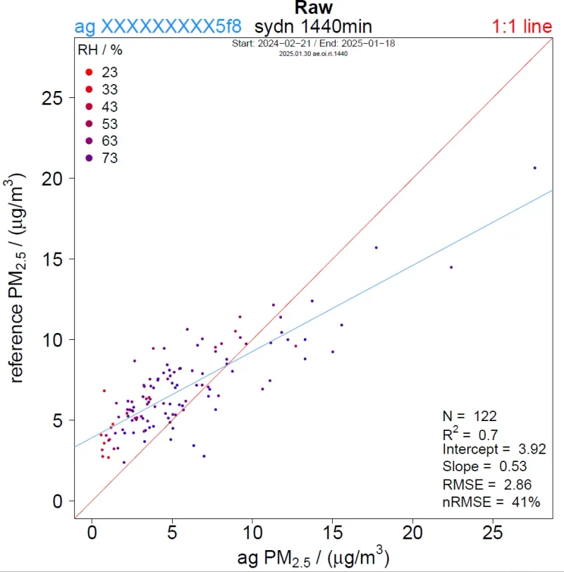
The reported PM_2.5 concentrations in Sydney were mainly below 10 µg/m³.

The reference instrument is based on beta attenuation, which has been reported to be subject to increased noise when PM_2.5 is low. We observed this behavior for all locations where we have beta attenuation references at such low concentrations (see scatter plots for Anacortes, Bellingham, and London Marylebone Rd in the appendix of this article). At these concentrations, a substantial fraction of the difference between reference and low-cost sensor is caused by the reference’s noise. If only looking at PM_2.5 concentrations higher than 10 µg/m³, we find an improvement through the EPA algorithm in Sydney.

Guatemala City (Guatemala)

We have two sensors collocated with a reference in Guatemala City. Each sensor gave us 21 days of colocation data, where reference data was available. The plot below shows a timeline with hourly data of the 2 x 21 days. The reference is shown in red, while the two AirGradient monitors are shown in blue. We currently cannot verify what reference instrument is in place here, so this location should be interpreted with care.

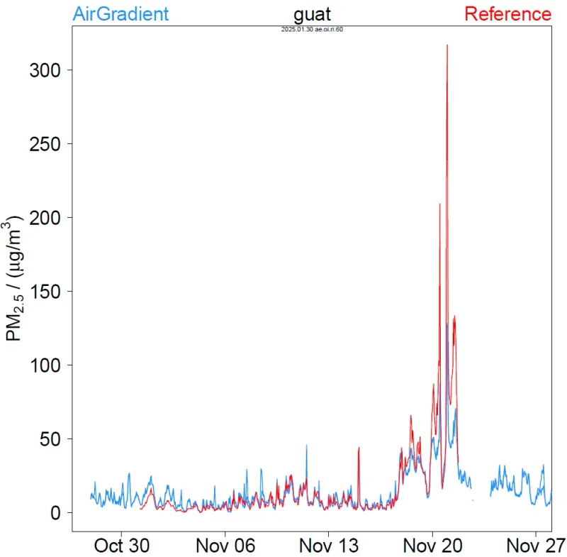
At the beginning of the 22 days, we can see that the AirGradient monitors tended to report higher readings than the reference. The opposite is the case at the end of the 21 days, where very high readings of >100 µg/m³ were reported by all three instruments. We find it hard to evaluate which of the two behaviors is more representative of this location, given that only 21 days are available. Note that both metrics MAE and RMSE are more sensitive to high than low PM_2.5 concentrations, implying that the end of the 21 days dominate MAE and RMSE.

Bogota (Colombia)

Two OpenAir monitors are collocated with a Thermo FH62C14-DHS in Bogota (Colombia). We have 38 and 31 days of collocated PM_2.5 data, partly shown in the timeline below (hourly data). The reference is in red, and the raw readings of the two AirGradient monitors are shown in blue.

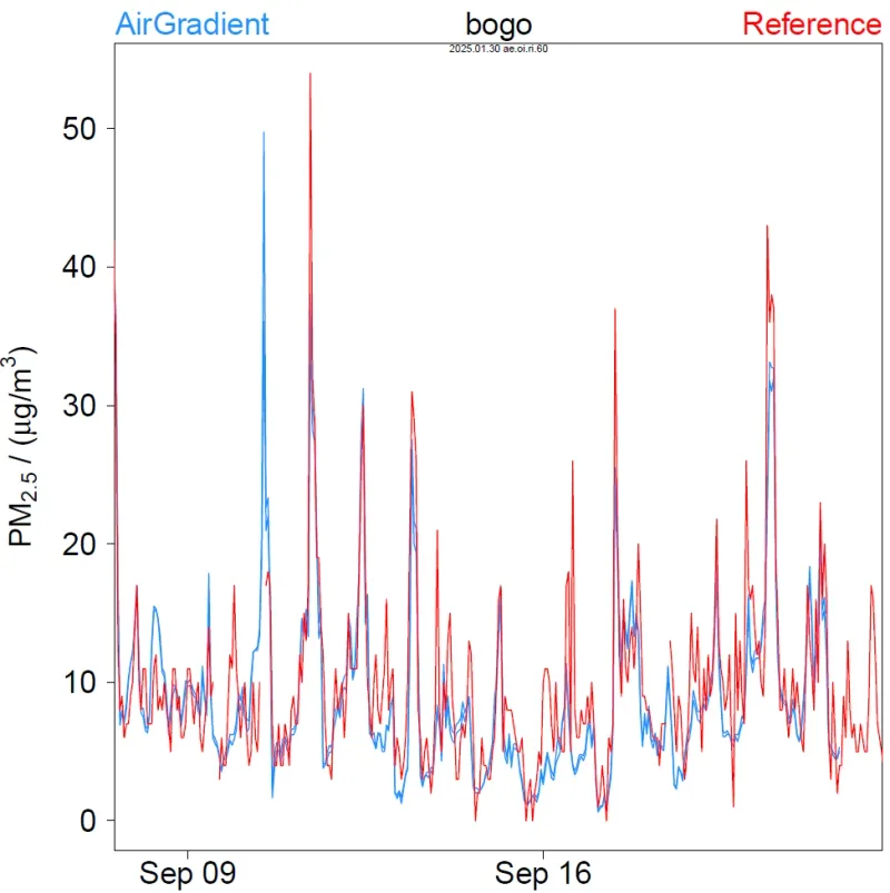
In Bogota, we already observe a good agreement between the raw AirGradient readings and the reference. The EPA algorithm decreases the PM readings and leads to an increased difference between AirGradient and reference. We have no verified explanation for that. It could be related to the reference instrument or the ambient aerosol. Note that Bogota is the only location where we test with a Thermo FH62C14-DHS, so we do not know how this reference normally compares to our monitors.

We have found a document from the US EPA where daily PM_2.5 readings from a Thermo FH 62 C14 were compared with FRM results. FRM refers to ‘Federal Reference Method’ and can be considered to be the most accurate. According to that document, the Thermo instrument overestimates the PM_2.5 concentrations by 60% in a chamber test with ammonium sulphate (Phase I, cf. Landis et al.). In other words, the Thermo instrument itself seems to overestimate, which needs to be considered.

Fun fact: We interpret the document above as the Thermo having overestimated PM_2.5 on average by a factor of 1.6 for ammonium sulphate. We normally observe such an error for our own monitors, which would explain the good agreement with the Thermo.

It could be that the Plantower PMS5003 sensors are factory calibrated using a Thermo FH 62 C14 or another reference that overestimates ambient PM in a similar fashion. This could explain the systematic overestimation of PM readings from the Plantower sensors.

Conclusion

Today’s article repeated the analysis from last September to assess the performance of EPA’s correction algorithm for raw PM_2.5 readings from AirGradient. This time, we have used more data from more locations.

The findings from last year could be confirmed: the algorithm significantly improved our PM_2.5 sensor accuracy, at least in 14 of 17 outdoor locations. In three locations (Sydney, Bogota and Guatemala City), an increased average difference between AirGradient and reference was observed as a result of the algorithm. However, this may be attributed to limitations of the reference instruments (high noise in the reference signal in Sydney, unknown reference instrument in Guatemala, and overestimating reference instrument in Bogota).

Today’s analysis emphasizes three aspects:

1. On average, the raw AirGradient PM_2.5 readings tend to overestimate ambient PM by approximately 50% at concentrations higher than 10 – 20 µg/m³.
2. On average, the EPA PM_2.5 algorithm improves the accuracy of AirGradient monitors for ambient PM as it accounts for aspect 1.
3. The choice of reference instrument should be taken into account when evaluating collocation data.

The Appendix can be downloaded here.

The data this article is based on will be available for download soon.

A big thank you goes to everyone who supported this study by co-locating our sensors and providing reference data:

• Northwest Clean Air Agency, USA

• Aire Ciudadano

• Université catholique de Louvain (UCLouvain), Belgium

• Sri Ramachandra Institute of Higher Education and Research (Deemed to be University), India

• National Astronomical Research Institute of Thailand

• Environment and Climate Change Canada

• Swiss Federal Laboratories for Materials Science and Technology (Empa)

• University of Washington / US Embassy Guatemala

• Imperial College London, UK

• Columbia University, USA

• The National Council for Air and Stream Improvement (NCASI), USA

• University of Sydney, Australia

• University of Cambridge, UK

• North West University, South Africa

• University of Manchester, UK