Beyond the numbers: the practical dilemma of size

This article is part of a series, where we explore the hidden complexities of PM2.5 — tiny airborne particles that impact air quality and health. We will uncover the ambiguities behind its measurement, the challenges in assessing health risks, and the surprising insights that emerge. Each article will tackle a different aspect of PM2.5, shedding light on its hidden dilemmas and unanswered questions. Today’s article discusses the practical challenges of defining particle size (in contrast to the last article, where we covered the theoretical challenges of size). We will compare how we want it to work in theory and how it looks in reality.

Introduction

As shown in the last article, there is a fundamental dilemma when expressing the size of a 3-dimensional particle using a 1-dimensional metric such as micrometer: it is not possible, unless our particles are perfectly spherical or cubic, but that’s not the case. We introduced the concept of ‘aerodynamic diameter’ which solves that problem, at least from a theoretical point of view. But is the size dilemma now really solved? Or do we have some more real-world limitations?

Size separation: How we want it to be

Let’s summarise what we have so far according to most definitions: PM2.5 refers to the mass of airborne particles with aerodynamic diameters smaller than 2.5 micrometers.

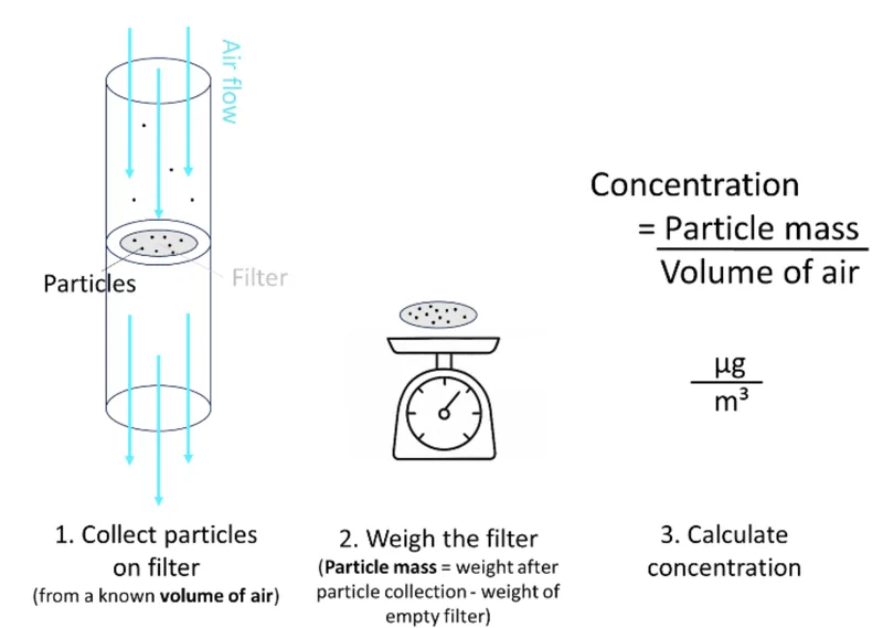
How can we measure the mass of these particles? Using a pump, we can let the air pass through a filter (see Figure 1). The particles in the air would thereby be collected on the filter. Putting the filter on a balance reveals the total mass of particles that were collected. We know the collection time and we know the air flow that prevailed during that time period, so we can easily calculate the total volume of air that went through the filter. Taking the previously measured mass and dividing it by the volume of air gives us the particle concentration in µg/m3.

But how can we make sure that only particles with aerodynamic diameter smaller than 2.5 µm are deposited on the filter? I mean there are also bigger particles that would heavily bias our measurement if they were deposited too.

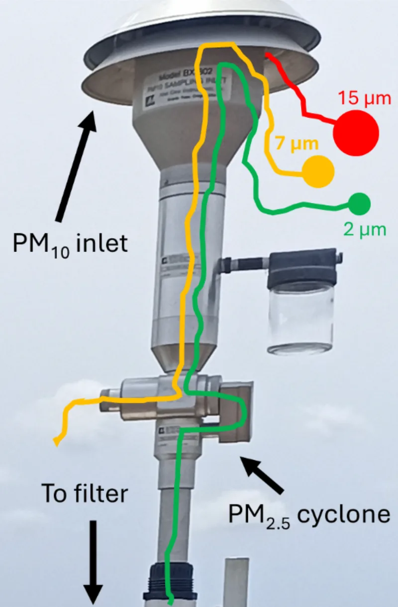
The trick is to use special sampling inlets before the air reaches the filter (see Figure 2). These inlets have a very specific geometry, which causes the incoming air to accelerate. Smaller particles remain in the air flow, while bigger ones start to deposit in the inlet due to inertia: big particles do not make it round the bend. Based on the geometry and the air flow, the manufacturers can control the size cut-off => bigger particles do not reach the filter and are excluded in the PM2.5 or PM10 measurement. Figure 2 shows an example of a PM10 inlet in combination with an in-line PM2.5 cyclone. A cyclone in PM monitoring is a device that separates larger particles from the air before measurement, and it’s called a cyclone because it uses a swirling, cyclone-like airflow to do this. The setup in this example only measures PM2.5 and not PM10.

Good news: the separation of smaller and bigger particles inside the sampling inlet of Figure 2 depends on the aerodynamic properties of the particles, and hence on the aerodynamic diameter. In conclusion, these techniques separate PM based on aerodynamic diameter and are therefore comparable with the EPA or WHO guidelines.

Size separation: How it is in reality

The previous section describes ideal size separation. However, the reality is different. Why? Because even with a perfect sampling inlet, it will not be possible to perfectly separate particles below/above a certain aerodynamic diameter. In fact, the imperfection can be quite drastic. In reality, there will always be some particles that make it through the inlet although they are bigger than the size cut-off, while some smaller particles are ‘incorrectly’ deposited in the inlet. See example below.

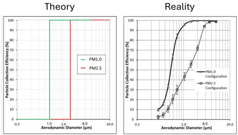
Figure 3 shows particle collection efficiencies i.e. what fraction of particles of a certain size gets stuck in the inlet and does NOT reach the filter / detector.

In an ideal world, all particles smaller than 1 μm (for PM1) should reach the filter, i.e. 0 % should be removed by the inlet, hence we should have 0 % particle collection efficiency below 1 μm. All particles above 1 μm, however, should be removed by the inlet, hence we should have a 100 % collection efficiency for all particles above 1 μm.

In practice, this looks very different (see Figure 3 right). For example, we see that at 2.0 μm, ca. 40 % of the particles do not make it through the PM2.5 inlet, although PM2.5 is defined as all particles smaller than 2.5 μm. On the other hand, ca. 95 % of the 2.0 μm particles do not make it through the PM1 inlet, while 5 % will reach the filter and contribute to the PM1 measurement although the particles are bigger than 1 μm.

We can also find a ca. 100 % - 95 % = 5 % probability of a 6 μm particle to end up in the PM2.5 fraction, although such a particle is clearly bigger than 2.5 μm. Note that one spherical particle with aerodynamic diameter of 6 μm is 14 times heavier than one 2.5 μm particle with the same density and shape. That might seem surprising but can be explained as the volume of a sphere, and hence its mass, is a cubed function of diameter. This emphasizes the influence of the size cut-off on the measurement and the importance to get it right.

As a result of this practical limitation, PM1, PM2.5 and PM10 are not simply defined as “ALL particles smaller than 1, 2.5 or 10 μm and NO particles above this size”. Instead, size cut-offs are usually defined with 50 % penetration efficiencies. For instance, in the case of PM2.5, 50 % of 2.5 μm particles make it through the inlet, while the remaining 50 % are excluded. This is accounted for in the definitions from EPA or WHO. It is counterintuitive, but this means that PM2.5 normally also includes particles with aerodynamic diameters above 2.5 μm. Confusing, right?

There is usually a maximum particle size defined for PM2.5 or PM10. It is typically 15 μm for PM10, but it really depends on the definition. Unfortunately, the term PM2.5 is often used without definitions, or the definitions are unclear. Additionally, it is often not well understood how different aerosols behave in different sample inlets (remember how different their shapes and materials can be). This highlights the real-world uncertainty that emerges as a consequence of the attempt to separate particles of different sizes.

Note that the same is also true for our lungs: although it is believed that particles with aerodynamic diameters of less than 10 micrometers reach the lungs, larger particles can also do so, the probability is just lower. This further highlights that PM2.5 as a health standard is characterized by a spectrum with many shades of gray rather than just black or white.

Conclusion

The previous article highlighted the fundamental limitation behind the desire to assign a one-dimensional particle size to an irregularly shaped particle. Although the introduced aerodynamic diameter solves that problem, it does not solve the real-world challenge of imperfect size separation. In consequence, we have to extend our definition of PM2.5 as follows: “PM2.5 describes airborne particles with aerodynamic diameters smaller than 2.5 μm based on a size separation with collection efficiencies as shown in a certain plot”. And then we would have to show a plot to explain what size separation we are referring to. That’s quite complicated, isn’t it? How shall we accurately measure something, if we have already such a hard time defining what we want to measure?

In practice, this ambiguity doesn’t make PM2.5 data meaningless, it simply reminds us to interpret them with care. The “2.5” is not an absolute boundary but a statistical one. Even the most precise instruments and standards, including those by the WHO and EPA, have to work within this blurred reality. Understanding this helps us appreciate both the strengths and the limitations of PM metrics and why comparing numbers across instruments or locations is never as simple as it seems.