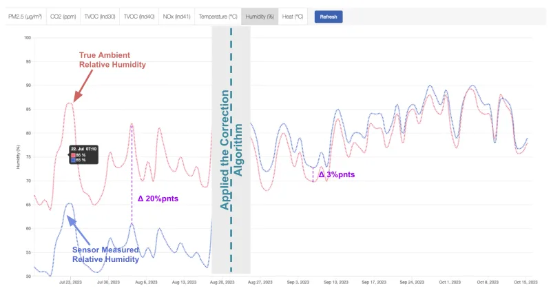
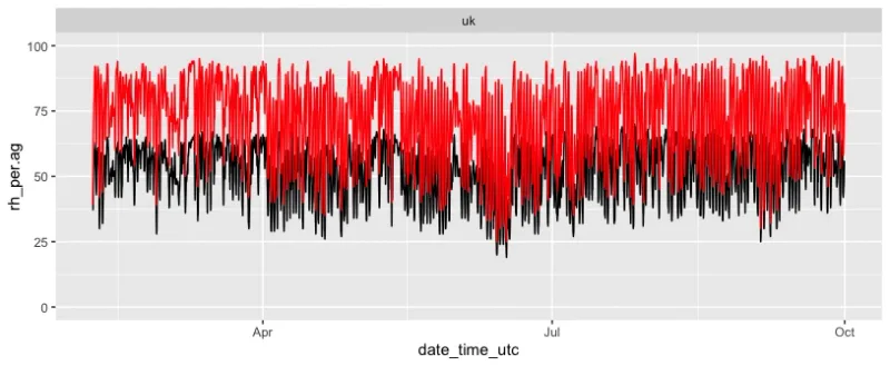
In August this year we applied an algorithm to improve the relative humidity (RH) accuracy measured in our particulate matter (PM) sensor. This reduced the gap to the true ambient humidity from about 20%pnts to less than 3%pnts. You can see this improvement effect very well in below chart.
This article will explain in detail how we developed this algorithm.
Analysing the Sensor
You might know that we use the Plantower PMS5003T PM sensor for our open-hardware outdoor monitor Open Air. The "T" in the model name indicates that it has a built-in temperature and humidity sensor. We specifically chose that model because measuring the humidity at the exact point where the laser does the PM measurement could give us advantages when developing a compensation algorithm on the PM measurement.
When testing the PMS5003T model against reference instruments, we very quickly noticed that the relative humidity measured by the PMS5003T was approximately 20%pnts below the real ambient relative humidity. You can see this very well in below chart where the PMS5003T is in black and the real ambient relative humidity from the reference instrument is in red.
But we can also see that the correlation appears to be very good. To check the correlation, it makes sense to make a x/y plot and calculate the R2 as a quantitative indication of the strength of the correlation. A number close to 1 in the R2 indicates a strong correlation and a number close to 0 no correlation.
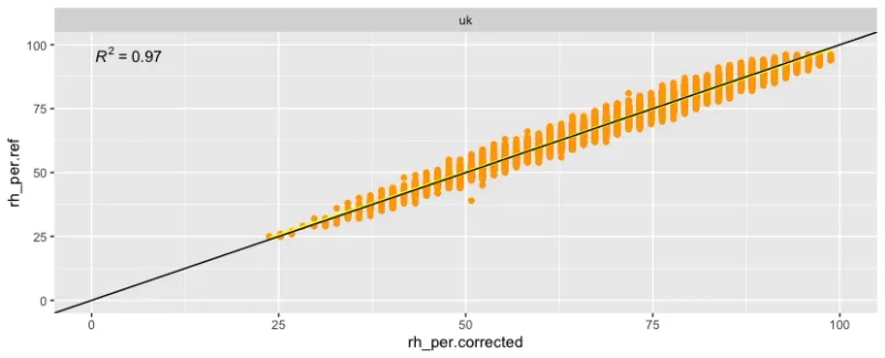
In the below x/y plot, you can see the RH for the PMS5003 sensor on the x-axis and the RH of the reference on the y-axis. So if a dot would be exactly on the black line, it would mean that the reference and PM5003 relative humidity is exactly the same.
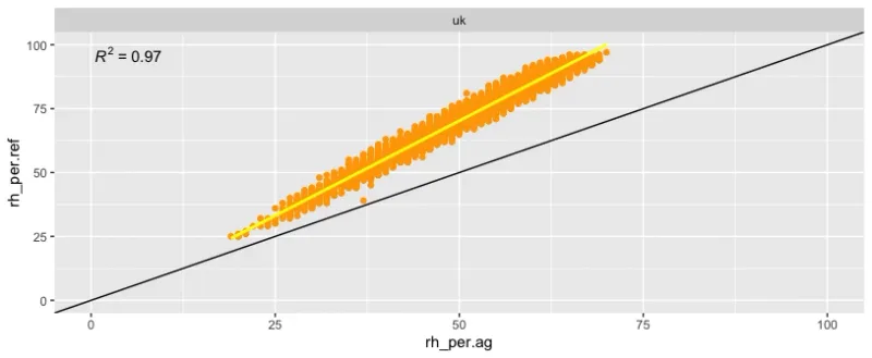
What we can see above is a very strong linear correlation with an excellent R2 of 0.97. However, we see also the strong underreporting by the PMS5003T sensor. So for example 50% relative humidity on the PM sensor is in reality around 70%.
This offset can also be calculated. Often a good metric for this is the RMSE (root mean square error). It measures the average difference between values predicted by a model and the actual values. In above case the RMSE of the raw data is 21.76. So this means that on average the PMS5003 relative humidity is a whopping 21% lower than it should be. Ideally we want the dots all around the black 1:1 line which would indicate that the PM sensor and the reference instrument measure exactly the same relative humidity levels.
Now let's fix this.
Using Linear Regression
There a many methods to come up with correction algorithms. From simple factors to black box AI / machine learning models. Since we see in above chart a very strong linear correlation, we will use one of the simplest method, a so-called "linear regression". Linear regression models describe the relationship between variables by fitting a line to the observed data.
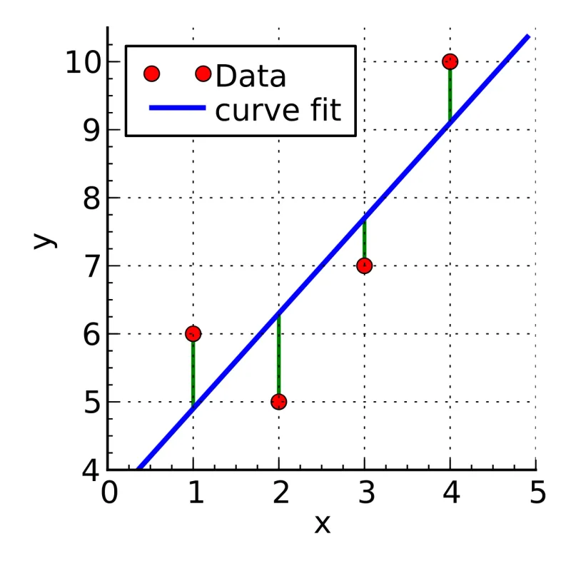
Linear regression models are often fitted using the least squares approach. The method works by minimizing the sum of the offsets or residuals of points from the plotted curve. So in below example it would be minimizing the green lines.
If you like to get deeper in how exactly linear regression is calculated, you can read the Wikipedia article.
Testing and Validation Set
When developing correction factors, it is important to separate the data set into a testing and a validation data set. If you don't, your results will be biased, and you'll end up with a false impression of better model accuracy.
So in our case we take approximately the first seven weeks (2023-02-06 to 2023-03-31) as training set and then calculate the fitting line. This fitting line we can actually already see as the yellow line in above chart. Now we just need the factors to move the yellow line above the black line. For this we need exactly two factors, an offset and a scaling factor.
We can then calculate the corrected relative humidity in the following way:
RH corrected = RH measured * factor + offset
To find the factor and offset we can use the statistical language R with just one line of code:
model_rh <- lm(rh_per.ref ~ rh_per.ag, data = data_training)
As you can see above, we do this only for the training set data.
In our case we do get a factor 1.500574 and an offset of -4.76.
So our exact correction formula would be:
RH corrected = RH measured * 1.500574 -4.76
Now we use this formula on all the data points collected by the PMS5003 sensor encompassing the whole data set and not only the training period.
If we plot the same charts as above we see that the corrected data from the PM sensor matches very very closely the reference data:
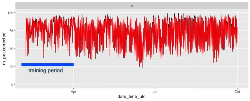
Important to point out is that we see the same good agreement on the complete timeline and not only during the range that was used for the training data.
On the xy chart, the yellow regression line now nearly fits the 1:1 line.
When we calculate the RMSE with the corrected value, we get a very good value of only 2.5. This means that the average error in relative humidity improved from 21.76 to only 2.52%pnts.
Validating the UK derived Algorithm in Thailand
Now there is one more thing we need to test before we apply these correction factors universally. Do they also apply to other climate zones and monitor locations?
For this we will travel around 6000 miles from the UK to Thailand.
At a school in Bangkok we have the same setup as the monitors in the UK and for the uncorrected data we see a very similar picture.
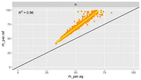
The R2 is also very good with 0.96 and a pretty bad RMSE at 20.001. Now we will use the same correction formula that was derived with the UK data: RH corrected = RH measured * 1.500574 -4.76.
What we see is a much improved data. The RMSE of the corrected data is now dramatically reduced to 2.94.
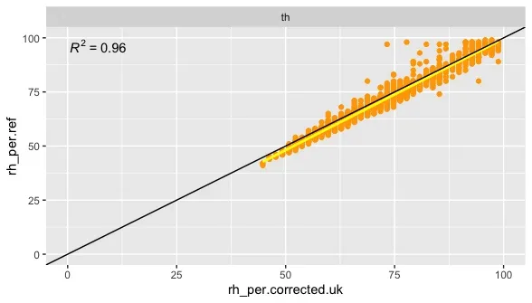
However, what we also see is that the yellow line is slightly below the black line. So probably having the data trained specifically with reference data in Thailand could have improved the results slightly.
If we do this and run the model specifically trained for the Bangkok data we can get a slightly better RMSE of 2.61. However, it is only an improvement of 0.33%pnts relative humidity and thus in most cases probably not relevant.
Here is a small overview table about the improvements with the linear regression model.
| Location | Error Before Correction | Error After Correction UK Algorithm | Error After Correction Local Algorithm |
|---|---|---|---|
| UK | 21.76 | 2.52 | 2.52 |
| Thailand | 20.00 | 2.94 | 2.61 |
Conclusion
Above demonstrates that you can dramatically improve the accuracy of sensors by using a simple linear regression model provided that your have a linear bias in your data. The example demonstrated is very typical and we see for example many air quality monitors reporting too high temperature because of the heat generated by the electronics in the enclosure. Above approach can help to improve these measurements.
As you can see from the data above, we did not yet cover a whole year so the algorithm might miss some seasonal variability. We will need to redo the analysis after a complete year to check for that.
I'm planning to write a follow-up article about how to actually calculate above in R with the complete data set and script so that people not familiar with the actual calculation can do this for their own data.