On November 25th, Achim posted a detailed description how to use R and RStudio to develop a linear regression correction algorithm. Today’s post is a practical example of how such a linear correction can be applied to real data.
Recently, one of our customers in Denmark approached us and emphasized that our OpenAir monitors overestimate temperature in cold environments – a systematic deviation, which we have seen in other locations too. We are aware of that inaccuracy and we currently collect data from more locations and seasons to develop appropriate correction algorithms. The reason for this deviation is that the electronic components inside the PM sensor heat up the air that is flowing through it. So, let’s develop a simple linear correction model based on the data from Denmark. First, let’s take a look at the raw data from Denmark to understand the problem:
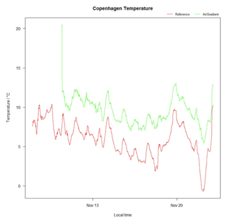
The figure above shows temperature over time reported by the OpenAir monitor in green and the reference monitor in red. Don't worry about the first few data points on the green line, as the OpenAir was probably first indoors before being set up outdoors. In consequence, the green and the red line should perfectly align as they both are the result from temperature measurements at the same location.
However, they do not align. The green line is systematically higher than the red one, on average roughly 3 °C. The temperature from the reference should be accurate enough to be considered as the true temperature, so there is only one reasonable explanation for what’s going on here: the temperatures measured by OpenAir monitors are approximately 3 °C higher than the true temperature – at least within the data set presented here.
Can we just substract an offset?
So can we just go ahead and subtract 3 °C from the Open Air monitor to get the true values? Before we do that, let’s take a look at another comparison between OpenAir and a reference. This time in Cambridge, England:
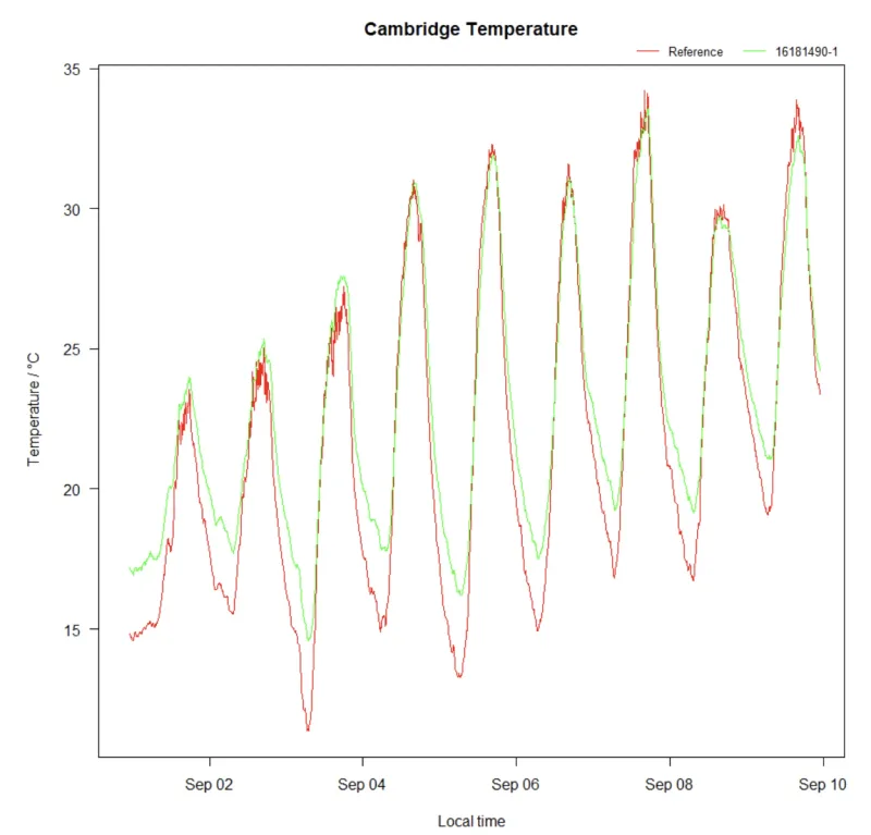
The figure above seems to have a much better alignment between OpenAir and reference. However, when we look more carefully, especially at lower temperatures, we find the same deviation of 3 °C as we have seen before. But this data set shows that the temperature deviation is not always 3 °C. Although it would be accurate to subtract 3 °C at lower temperatures, it would be inaccurate to do that at higher temperatures. Where is the line between low and high temperatures? So now we realise that it takes a bit more than just subtracting a fixed number. In order to correct our temperature readings, we need something more sophisticated.
Deep dive into the Data
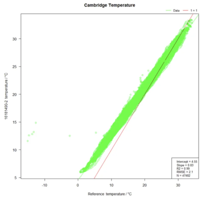
In the figure above, we have summarized the temperature data from roughly 165 days in Cambridge, England. Note, the plotting has changed as the x axis is no longer time. Instead, the x axis now represents the readings from the reference and the y axis represents the readings from the OpenAir.
Every green point illustrates a timepoint within the 165 days and shows what temperature has been measured by the reference and by OpenAir for this specific timepoint. Ideally, all green dots perfectly align with the red 1:1 line. In such a case, there would be no difference at all between the OpenAir and reference readings. The figure shows that the green dots indeed follow a line, but the line is a bit less steep and on average a bit higher than the ideal red line. For example, at a reference temperature of 10 °C, we can see that OpenAir on average reports 13 °C. This is in line with the systematic deviation of 3 °C we have found in the previous figures for low temperatures.
At the same time, we can see that for high temperatures of for example 30 °C, the OpenAir readings are roughly 1 °C below the reference. According to the data from Cambridge, temperature accuracy of OpenAir is at its best around 25 °C, where the green line intersects the red line. All that information that we describe here in text format are basically already the information we need for the temperature correction. However, we need it in a numerical format in order to apply the model. So what is the correction formula now?
Some more information is shown in the small box at the bottom right hand side of the previous figure. We see an intercept of 4.55 and a slope of 0.83 resulting from the linear model calculated in RStudio, as described by Achim in his post. The intercept indicates where the green line intersects the x axis. In other words: that’s the temperature reading of the OpenAir when the reference reports 0 °C. The slope of 0.83 shows what we already knew before: the green line is less steep than the red one. But now we exactly know the steepness: 0.83.
Assuming the performance of OpenAir in Cambridge is the same as in Denmark, we can use the following functional equation for temperature correction:
Temperature OpenAir=0.83 x Temperature Reference + 4.55°C
Note, all temperatures must be in degrees Celsius, otherwise the slope and intercept will be different. Solving equation above for reference temperature results in:
Temperature Reference= (Temperature OpenAir - 4.55°C) % 0.83
And that’s it, the equation above is the linear correction model for the OpenAir temperature! We simply take the OpenAir reading, subtract 4.55 °C and divide by 0.83. Theoretically, this should give us fairly accurate temperatures within the temperature range of the Cambridge data. Let’s try to verify our model using the Denmark data.
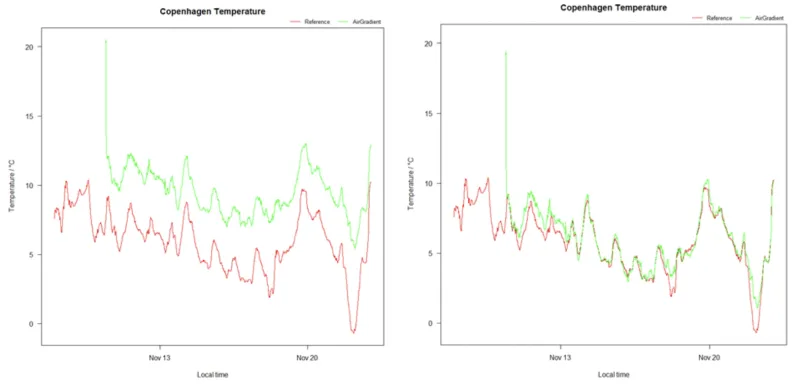
The two figures above show the measured temperatures by OpenAir (green) and reference (red) in Denmark. The OpenAir data on the left is raw, whereas the OpenAir data on the right has been corrected using the linear algorithm described in this post.
As you can see, the alignment between red and green improved significantly, supporting the validity of our model. Now, OpenAir’s temperature accuracy is almost the same as the one from the reference. However, to properly verify this model we would have to consider other temperature ranges and locations too. We can do that for the location in Denmark once more data is available. Generally: the more data available, the more accurate correction algorithms can be developed and the more profound verifications can be undertaken.
Important: Before we come up with globally recommended temperature correction algorithms we need more data across broad temperature ranges, various locations and all seasons of the years. We will keep you informed as we introduce these more general correction algorithms.
If you have some data that you think could help us developing these, please feel free to share with us!