Nitrogen dioxide (NO2) is one of the most common and dangerous urban air pollutants. This reactive gas is primarily formed during high-temperature combustion processes, in which atmospheric nitrogen reacts with oxygen at extremely high temperatures. Its major sources include vehicle emissions, industrial sectors, power plants and indoor gas appliances such as stoves. Even at low concentrations, NO2 causes respiratory problems and lung inflammation, affecting asthma and COPD, particularly in sensitive populations such as children and the elderly. Aside from these direct health risks, NO2 performs as a precursor in atmospheric reactions that produce toxic surface ozone (O3) and fine particulate matter (PM2.5), causing substantial environmental impacts such as acid rain and aquatic eutrophication.
AirGradient developed the AirGradient Open Air Max monitor to provide accurate, community-driven and open-source data. To ensure that our low-cost monitors deliver research-grade accuracy, we have integrated a calibration pipeline. By pairing our electrochemical NO2 sensors with a reference NO2 analyzer in our calibration chamber, we apply correction algorithms to make our data reliable and accessible.
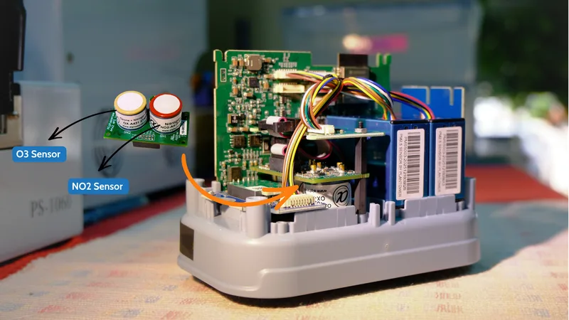
The AirGradient Open Air Max utilizes an electrochemical sensor (Alphasense A43F) as well as a separate ozone (O3) sensor to subtract cross-sensitivity. However, hardware alone is insufficient; precision and accuracy may only be obtained by calibration.
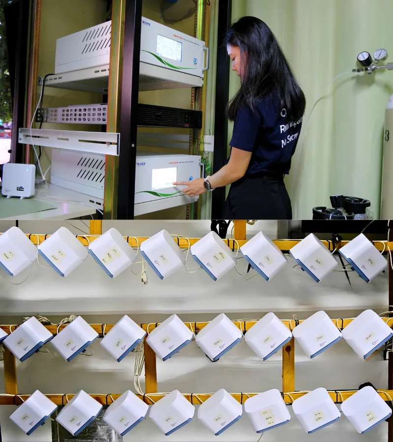
To calibrate these sensors, we set up a chamber room with an FPI AQMS-600 Nitrogen Oxides Analyzer. The AQMS-600 is a federal reference instrument that uses the chemiluminescence detection method, which is the gold standard for regulatory monitoring. Nitric oxide (NO) interacts with Ozone (O3) to form reactive state NO2 molecules, which emit light in proportion to concentration. The instrument is highly accurate, accounting for detecting concentration variations down to parts per billion (ppb) levels.
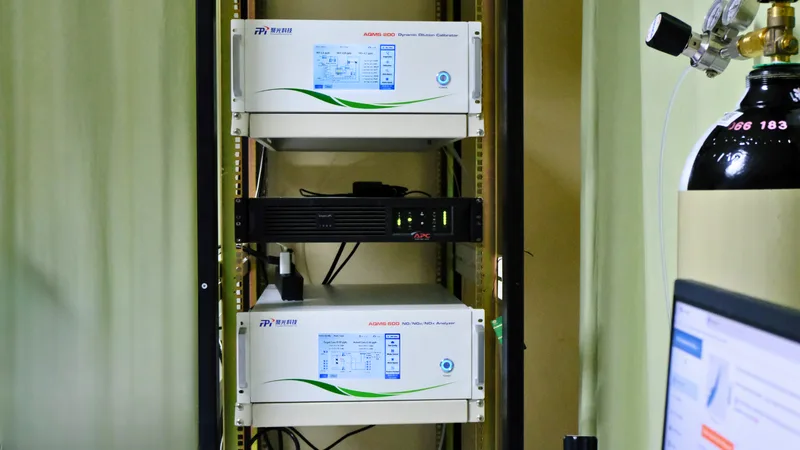
Before we ship the AirGradient Open Air Max monitor, we place it in our chamber alongside the AQMS-600 analyzer. We systematically cycle through known NO2 concentrations. By comparing the raw electrochemical voltages (mV) which are converted in ppb and the absolute concentrations recorded by the AQMS-600, we perform our high-resolution factory calibration.
The calibration methodology that we performed by using the linear-regression algorithm. Calibration concept is based on simple linear regression between co-located sensors and reference instrument using following equation:
Reference readings = LCS readings x correction coefficient (slope) + offset (intercept)
Once calibration parameters were obtained, then applied to new LCS readings to obtain corrected concentrations. Corrected concentrations could be compared to co-located reference readings for validation of calibration. Moreover, this simple linear regression can be replaced with multi-linear regression in the future, taking into account variation in temperature and relative humidity.
Influence of temperature and relative humidity on the sensitivity of the sensors.
Methodology: For each sensor unit, a series of ordinary least squares regression models was developed to evaluate the influence of meteorological variables on sensor calibration performance. The corrected sensor signal was first calculated as the difference between the working electrode and auxiliary electrode signals:
S=WE-AE (1)
Where;
S is corrected sensor signals (mV)
WE is working electrode signals (mV)
AE is auxiliary electrode signals (mV)
Temperature and relative humidity were mean-centered prior to model development:
Tc=T-Taverage (2)
Where;
TC is temperature mean-centered (celsius degrees)
T is temperature (celsius degrees)
Taverage is average temperature (celsius degrees)
RHc=RH-RHaverage (3)
Where;
RHC is relative humidity mean-centered (%)
RH is relative humidity (%)
RHaverage is average temperature (%)
Centering was applied to improve the interpretability and numerical stability of the regression models, particularly when interaction terms were included.
Several calibration models with increasing complexity were tested for each sensor. The simplest model included only the corrected sensor signal. Additional models included temperature and relative humidity either as additive predictors or as interaction terms with the sensor response. The tested models are listed in Table 1, where ref is the reference NO2concentration, S is the corrected sensor signal, k is the corresponding regression coefficient, and b is the intercept.
Table 1 Linear regression models for prediction of NO2 concentrations
| Model | Included parameters | Equation |
|---|---|---|
| M1 | sensor only | Ref=k🇸S + b |
| M2 | sensor, temperature | Ref=k🇸S +k🇹T+ b |
| M3 | sensor, humidity | Ref=k🇸S +k🇷🇭RH+ b |
| M4 | sensor, temperature, humidity | Ref=k🇸S +k🇹T+k🇷🇭RH+ b |
| M5 | sensor, temperature, sensor * temperature interaction | Ref=k🇸S +k🇹T+k🇸 🇹ST+ b |
| M6 | sensor, humidity, sensor * humidity interaction | Ref=k🇸S +k🇷🇭RH+k🇸 🇷 🇭SRH+ b |
| M7 | sensor, temperature, sensor * temperature interaction, sensor * humidity interaction | Ref=k🇸S +k🇹T+k🇷🇭RH+k🇸 🇹ST+k🇸 🇷 🇭SRH+ b |
A time-based 70/30 train–test split was used to evaluate the predictive performance of the calibration models. The first 70% of observations for each sensor were used for model fitting, and the remaining 30% were used for independent testing. The dataset covered the period from 22 June 2026 17:00 to 23 June 2026 16:59 and included 15,870 valid 3-min observations from 30 sensor units. The number of observations per sensor ranged from 472 to 643, with an average of 529 observations per sensor.
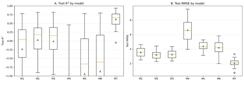
Results: The initial model comparison was performed using in-sample fit metrics to evaluate how different regression structures described the calibration dataset. The sensor-only model showed moderate explanatory power, with R2 values ranging from 0.586 to 0.843 across the sensors. After including temperature, relative humidity, and sensor–meteorology interaction terms, the in-sample model performance improved substantially. For the M7 model, R2 values ranged from 0.908 to 0.975, with all 30 sensors achieving R2 > 0.90. On average, R2 increased from 0.717 for M1 to 0.940 for M7, corresponding to a mean increase of 0.222.
A similar improvement was observed for the in-sample prediction error. The mean RMSE decreased from 5.66 for the sensor-only model to 2.62 for M7, corresponding to an average reduction of approximately 54%. Across individual sensors, RMSE decreased from 4.39–6.94 in M1 to 1.71–3.29 in M7. These results indicate that the inclusion of meteorological variables and interaction terms substantially improved the agreement between the sensor response and reference NO₂ concentrations within the calibration dataset. However, because these metrics were calculated on the same data used for model fitting, they should be interpreted as measures of model fit rather than independent predictive performance.
To evaluate model generalizability, a time-based 70/30 train–test split was then applied separately for each sensor. The first 70% of observations were used for model fitting, and the remaining 30% were used for independent testing. This validation step showed that the predictive performance was lower than the in-sample fit, as expected, but confirmed the advantage of the interaction-based model. Among all tested models, M7 achieved the best test-set performance, with a mean test R2 of 0.619 and the lowest mean test RMSE of 2.09.
The train–test results also showed that models containing only additive meteorological terms were not sufficient for robust prediction. In particular, the additive temperature and relative humidity model M4 performed poorly on the independent test period, indicating limited temporal generalizability. This suggests that temperature and relative humidity affect the sensor response primarily by modifying the sensor sensitivity rather than acting only as independent additive predictors.
The standardized regression coefficients of M7 provided further insight into the relative importance of the predictors. The corrected sensor signal had a consistently positive effect across all sensors, with a mean standardized coefficient of 0.328. The direct effects of temperature and relative humidity were less consistent between sensors. The standardized coefficient for temperature was positive for 18 sensors and negative for 12 sensors, while the coefficient for relative humidity was negative for most sensors.
The strongest and most consistent effect was observed for the interaction between the sensor signal and temperature. The standardized coefficient for the sensor–temperature interaction was negative for all 30 sensors, with a mean value of −3.159. This indicates that temperature systematically modified the sensitivity of the electrochemical sensor response. The sensor–relative humidity interaction was also generally important, with positive standardized coefficients for 28 of 30 sensors and a mean value of 1.209. Overall, these results indicate that M7 provides the best predictive performance and supports the interpretation that meteorological variables influence the electrochemical sensor response through changes in sensitivity.