This article is part of a series, where we explore the hidden complexities of PM2.5 — tiny airborne particles that impact air quality and health. We will uncover the ambiguities behind its measurement, the challenges in assessing health risks, and the surprising insights that emerge. Each article will tackle a different aspect of PM2.5, shedding light on its hidden dilemmas and unanswered questions. Today’s article discusses the accuracy of different reference monitors.
Introduction
In the previous episodes of Beyond the Numbers (found here, here and here), we explored why PM2.5 is more complex than it first appears. We looked at how particle size is not always straightforward to define and why a seemingly simple metric like “2.5 micrometers” hides assumptions about particle shape, density, and behavior in air.
This naturally leads to the next question:
When governments publish PM2.5 data, what exactly are they measuring? And what makes one monitor a “reference” monitor?
At first glance, the answer seems simple. Reference monitors are often seen as the gold standard: the instruments that tell us the true concentration of PM2.5 in the air. But in practice, things are more nuanced than they first appear.
A reference monitor does not measure the absolute truth. Instead, it measures PM2.5 according to an agreed method. That distinction may sound subtle, but it can have important consequences for how we interpret air quality numbers.
Measuring PM2.5: two fundamentally different strategies
Let’s first take a look at how reference monitors measure airborne particles. There are many types of PM monitors, but most fall into two broad categories:
mass-based monitors, which collect particles and determine their mass directly,
optical monitors, which detect particles in air using light and estimate mass indirectly.
Both approaches are widely used. Both can provide useful data. But they answer the question “how much PM2.5 is in the air?” in different ways.
Mass-based monitors: measuring what is being deposited
Mass-based monitors might be closest to what many people intuitively imagine.
Air is drawn through a size-selective inlet, which removes larger particles and allows only PM2.5 to enter. The particles are then collected on a filter or another surface. The instrument determines how much mass has accumulated.
The simplest version is manual filter weighing:
a filter is weighed before sampling,
air passes through it for several hours or a full day,
the filter is weighed again,
the mass increase is divided by the sampled air volume.
Many monitoring stations use filter-based mass measurements as the reference for PM2.5. This means someone has to go out to the site, swap yesterday’s filter for a new one, and bring the used filter back to a lab where it is weighed to determine yesterday’s PM level. Then the whole process starts again the next day with a fresh filter.
It’s easy to see why this is so labour-intensive. It requires regular (often daily) visits to each monitoring station, including weekends and holidays. This operational burden makes continuous manual monitoring impractical, especially at remote places.
The need for automated instruments is obvious. These systems follow the same basic principle: particles are drawn into the instrument and collected either on a filter substrate or directly onto a sensing element. The accumulated mass is then determined using different physical principles, most commonly beta attenuation monitoring (BAM) or tapered element oscillation microbalance (TEOM).
- Beta attenuation monitors (BAM)
These use a weak beta radiation source. As particles accumulate on a moving filter tape, they absorb part of the radiation. The reduction in signal corresponds to deposited mass.
- Tapered Element Oscillating Microbalance (TEOM)
These use a small oscillating element. As particles deposit, the element becomes heavier and its vibration frequency changes.
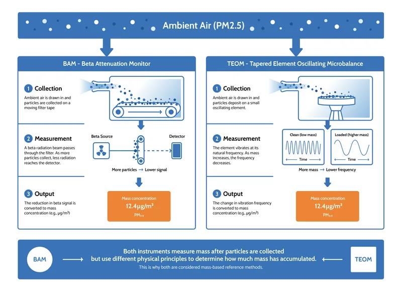
Although BAM and TEOM work differently, both still rely on measuring material that has physically been collected from the air. In that sense, they are mass-based approaches.
Advantages
- Direct measurements of mass. No assumptions about particle shape or density are needed.
Limitations
One monitor can only measure PM2.5 or PM10 (not both).
Particle size distribution is unknown.
Low time resolution
If a monitor reports PM every hour, enough mass must accumulate within that hour. This becomes difficult at low PM levels resulting in noisy readings. This limitation has become more relevant as ambient levels have declined in many countries since the PM standards were introduced in the 1980s.Differences in design and calibration can lead to systematic differences between manufacturers.
Optical monitors: measuring light, not mass
The second type of PM monitor relies on an optical phenomenon. This approach is used in a wide range of instruments, from reference-grade devices (e.g. from Grimm, Palas, Teledyne) to low-cost monitors (e.g. from PurpleAir, QuantAQ, TSI, AirGradient).
These monitors illuminate airborne particles with a laser (see Figure 2). A portion of the light is scattered by the particles and detected by a sensor. In simple terms: the more and the larger the particles, the more light is scattered.
Some instruments are designed so that particles pass through the laser one by one. This is called single-particle counting. Each particle produces a distinct signal (“pulse”) as it passes through the light (shown at the bottom right of Figure 2).
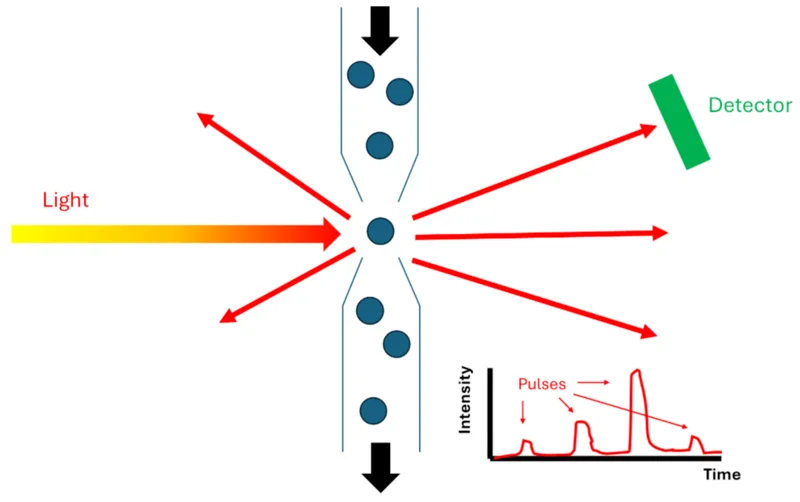
In the example shown, four particles are detected during the measurement period. Knowing the airflow through the instrument allows us to calculate the sampled air volume, which gives the particle number concentration.
Number concentration is useful, but it does not directly provide particle size or mass. Luckily, the intensity of the scattered light signal is related to particle size. To establish this relationship, the instrument is calibrated in the factory using particles of known size.
Once this relationship is known, each detected light pulse is converted into a particle size. From this, particle volume can be estimated assuming spherical particles. Volume is then converted to mass by assuming whatever density seems most appropriate for typical PM. In this way, a mass estimate is obtained for every particle detected by the laser.
Importantly, this is not a direct measurement of mass. It is an estimate based on particle volume and optical size, rather than aerodynamic size. As a result, the readings are not always directly comparable to regulatory standards such as WHO guidelines. This fundamental limitation applies to both reference-grade and low-cost optical instruments.
In summary, optical monitors do not directly measure PM mass. Instead, they count particles, estimate their size from the scattered light signal, and then infer mass based on assumed particle shape and density. In practice, this conversion depends strongly on the assumptions made during calibration and on the particles being measured.
Larger deviations can occur when real-world particles differ from those the instrument was optimised for. This is particularly relevant because ambient particles vary widely in shape and composition. Manufacturers apply correction factors to reduce these effects on average, but this “on average” matters: performance can vary depending on the actual mix of particles in the air at any given time.
Different manufacturers also use different designs and calibration approaches, which can lead to systematic differences between instruments even when they sample the same air.
Advantages
One monitor can measure both PM2.5 and PM10 at the same time
Particle size distribution is known.
No particle collection needed. The monitors can reliably provide PM readings even on a per second basis.
Limitations
Mass is not directly measured. Particle shape and density are assumed based on real-world testing. Different manufacturers make different assumptions (and often they are not disclosed).
Compared to mass-based monitors, optical monitors depend more strongly on particle type: accuracy is higher when particles match calibration assumptions, and lower when they do not.
How accurate are reference monitors?
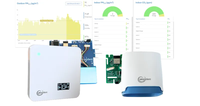
We at AirGradient use automated reference monitors (in our case an optical instrument from Palas) to test the accuracy of our low-cost sensors. This raises a basic question: how accurate are the reference monitors themselves? And who tests that?
Manufacturers of automated reference instruments (such as BAM, TEOM, or optical monitors) carefully test and validate their devices to ensure they provide accurate measurements. However, there is relatively little independent evidence showing whether different reference models actually agree with each other when measuring the same ambient air.
One reason for this is that manufacturers typically focus on testing and validating their own instruments, rather than directly comparing them against competing models from other companies.
In U.S. regulatory air quality monitoring, automated PM reference monitors are known as federal equivalent methods (FEM). They are typically compared against a more accepted “gold standard” called the federal reference method (FRM), which measures PM2.5 by collecting particles on filters over 24 hours and weighing them manually in a laboratory.
A 2024 study by Tanvir Khan and colleagues is one of the most comprehensive evaluations in this context. It examined 276 monitoring stations across the United States where both FEM instruments and FRM filter measurements were available, allowing a direct evaluation of the accuracy of the automated reference monitors.
The study assessed how closely FEM measurements matched the FRM values. In this type of comparison, values close to the horizontal line at 1 (Figure 3) indicate better agreement between the two methods.
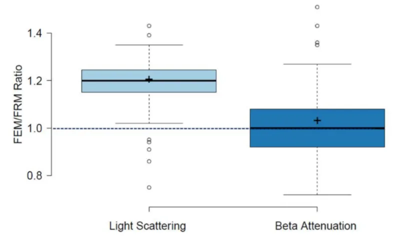
Assuming the filter weighing method is the most accurate, Figure 3 shows that optical reference instruments tended to overestimate PM2.5 by about 20% on average. In contrast, beta attenuation monitors (BAMs) were, on average, quite accurate. However, performance varied depending on location for both types of instruments. Some monitors read up to 34% too low on average, while others overestimated concentrations by as much as 44% on average.
These differences may not strongly affect trends if the same type of monitor is used consistently over time. However, they can become important when comparing pollution levels between different places. In such cases, a 20% difference between two locations may reflect real differences in air quality, but it may also simply result from different reference instruments at each site.
Why automated reference monitors still matter
Manual filter weighing is labour-intensive, expensive, and usually provides only a single measurement per day. It is often not feasible, especially in remote locations. Automated reference monitors help fill this gap by delivering continuous data, making it possible to analyse long-term trends, support regulatory decisions, and compare air quality across time and locations.
However, the term “reference” does not imply a perfect ground truth. It refers to standardized measurement methods that are accepted and intended to produce comparable results. The key word here is “intended”.
It is also worth noting that even manual filter weighing is not without limitations. In recent years, concerns have been raised about its accuracy at low PM concentrations, where only small amounts of material are collected on the filter and weighing uncertainty becomes more important. This is relevant in environments with relatively clean air.
Conclusion
PM2.5 readings are often presented as clear numbers, but in reality they are estimates within an uncertainty range. Mentioning the estimate without the uncertainty is like having one leg in boiling water and the other in freezing water, and then calling it a comfortable average.
As shown by Tanvir Khan and colleagues, federally approved reference monitors can differ from each other and from the filter-based “gold standard” by up to around 30%. This does not mean the instruments are wrong, but reflects the limits of measuring a complex mixture of airborne particles.
After decades of progress, PM2.5 can now be measured automatically with reasonable accuracy, but not with the level of accuracy seen for more uniform pollutants such as CO₂. This is expected, as PM2.5 is an umbrella concept that covers particles with varying sizes, shapes, densities, and optical properties. Importantly, health effects are not driven by PM2.5 mass alone, but also by the particle composition, which makes a mass-based, single-number metric inherently limited to begin with.
This makes it important not to over-interpret numbers. Reporting PM2.5 to two decimal places can suggest an accuracy that is not present. If low-cost sensors are within ±30% of a reference monitor, they are already within the range of disagreement reported between reference instruments themselves. This implies a limit to how accurate low-cost sensors can become, when the accuracy of the reference methods themselves becomes the bottleneck.
The complexity of monitoring PM2.5 is reflected in US EPA guidelines, which consider agreement within ±30% (nRMSE) and differences of up to 7 μg/m³ (RMSE) acceptable for daily PM2.5 measurements. This level of measurement uncertainty is relevant at low concentrations that are now common in many (though by no means all) countries.
Over the past 100 years, PM2.5 pollution has changed. Strict policies on combustion sources have decreased the dominance of combustion-related particles in many countries. The particle mixture has become more diverse, making both health assessment and air quality monitoring more complex. At the same time, PM2.5 levels have declined substantially in these places, to the point where WHO air quality guidelines for annual exposure are now at 5 μg/m³. The concentrations of health concern are approaching the level of uncertainty in the methods used to assess them. What does this mean for determining whether the WHO limit is met or not? And how does this discussion about confidence at low concentrations resonate in countries where 100 µg/m³ is a daily reality?